# Libraries
library(tidyverse)
library(tidymodels)

# Settings
theme_set(
  new = theme_classic()
  )
tidymodels_prefer()

# Import csv file
data <- read.csv("https://raw.githubusercontent.com/GeorgeOrfanos/Data-Sets/refs/heads/main/Datacamp_public_datasets/recipe_site_traffic.csv")

# Column Names
names(data) <- c("Recipe", "Calories", "Carbohydrates", "Sugar",
"Protein", "Category", "Servings", "High_Traffic")Recipe Site Traffic - A Data Science Approach
Introduction
In this case study, we discuss a data analysis approach for the Recipe Site Traffic project, based on the practical exam for the Data Scientist Professional Certificate from DataCamp.
According to the project description, a predictive model is needed that can predict which recipes are associated with high traffic in the website. The business case is that the product manager is interested in identifying which recipes attract more visitors. From a business point of view, higher traffic has the potential to lead to higher revenues.
For this purpose, a predictive model was needed that could do the following:
- Predict which recipes will lead to high traffic
- Correctly predict high traffic recipes
The written report was required to include the following sections:
Data Validation: Verifying the accuracy and quality of the data.
Exploratory Data Analysis: Examining the data to identify patterns and insights.
Predictive Modeling: Splitting the data into training and test sets, fitting two different types of predictive models and evaluating the results.
Final Summary and Recommendations: Providing a concise overview and actionable recommendations for the business.
For this project, we use the programming language R, along with the tidyverse and tidymodels frameworks. In the following sections, we present the graphs and code used in this analysis.
Data Validation
The dataset is provided in CSV format and consisted of 947 rows (observations) and 8 columns (variables). The following image displays the variable names along with their descriptions.

To begin the project, we load the necessary R packages and set the theme for the plots, and import the dataset. Also, we adjust the column names of the given data set to make it more specific to my needs.
The data set has 8 columns which are described below:
Recipe: Numeric, unique identifier of recipeCalories: Numeric, number of caloriesCarbohydrate: Numeric, amount of carbohydrates in gramsSugar: Numeric, amount of sugar in gramsProtein: Numeric, amount of protein in gramsCategory: Character, type of recipe. Recipes are listed in one of ten possible groupings (Lunch/Snacks’, ‘Beverages’, ‘Potato’, ‘Vegetable’, ‘Meat’, ‘Chicken, ’Pork’, ‘Dessert’, ‘Breakfast’, ‘One Dish Meal’).Servings: Numeric, number of servings for the recipeHigh_Traffic: Character, if the traffic to the site was high when this recipe was shown, this is marked with “High”.
From this dataset, the variable Recipe has no missing or suspicious values. However, we transform this column to a character type to be sure regarding the nature of this variable. The variable High_Traffic has either the value “High” or NA, which we substitute with the value of 1 if the value was “High” and 0 if it was NA. We also transform this variable to factor for the predictive modeling process later. Additionally, there are two observations in the variable Servings that although show the number of recipe servings, they also include the text “as a snack”, a text that was removed. Lastly, the variable Category includes the values “Chicken” and “Chicken Breast”, but according the description of the data set, there should be only the value “Chicken”.
Based on this description, we manipulate the data set to ensure the data type and initial values of every column.
# Data Cleansing
data <- data %>%
  mutate(Recipe = as.character(Recipe),
         Calories = as.numeric(Calories),
         Carbohydrates = as.numeric(Carbohydrates),
         Sugar = as.numeric(Sugar),
         Protein = as.numeric(Protein),
         Category = if_else(Category == "Chicken Breast",
                            "Chicken",
                            Category),
         Category = as.character(Category),
         Servings = str_replace(Servings, " as a snack", ""),
         Servings = as.character(Servings),
         High_Traffic = if_else(is.na(High_Traffic), 0, 1),
         High_Traffic = factor(High_Traffic, levels = c("1", "0")))
It is important to mention that the variables Calories, Carbohydrates, Sugar and Protein have NA values in about 5% of the cases. These missing values occur consistently across the same rows, meaning that if the column Calories has NA value, then the whole row has NA values in the other mentioned columns as well.
We leave these values as NAs for now since we use cross-validation in the predictive modeling process. The reason for this is to avoid any potential data leakage. For this imputation, we impute these numeric variables via a linear model with the variables Category and Servings.
Exploratory Data Analysis
The first move in the exploratory analysis is to check the values of the variable of interest. The graph below shows that the ratio of the recipes that leads to high traffic is approximately 60%. From a probability theory perspective, this means that if we pick randomly a recipe from the existing data set, then there would be 60% probability that the traffic would be high.
# High Traffic
data %>%
  count(High_Traffic) %>%
  mutate(Ratio = n/sum(n)) %>%
  ggplot(aes(x = High_Traffic,
             y = Ratio)) +
  geom_col(fill = "skyblue") +
  labs(x = "High Traffic")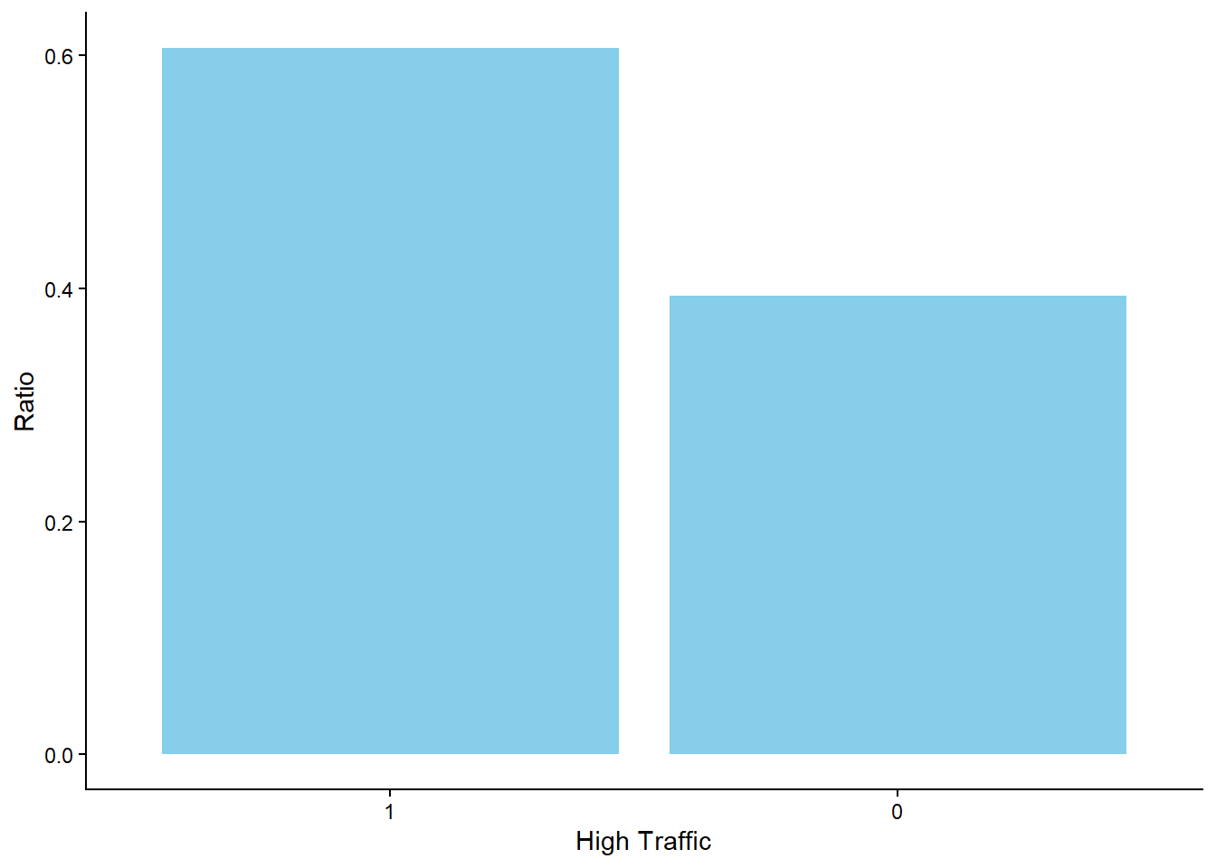
The graph below shows that the “Chicken” category captures the highest ratio of all the recipes (with 18%) while the “One Dish Meal” captures the lowest ratio with only (7.5%). Therefore, although the other types of meat are below 10%, we see that most recipes include chicken. Additionally, recipes such as “Breakfast” and “Beverages” are also relatively high, but still the difference seems to be significant between the ratio of the “Chicken” and any other category.
# Traffic within Category
data %>%
  count(Category) %>%
  mutate(Ratio = n/sum(n),
         Category = fct_reorder(Category, Ratio)) %>%
  ggplot(aes(x = Category,
             y = Ratio)) +
  geom_col(fill = "skyblue") +
  coord_flip()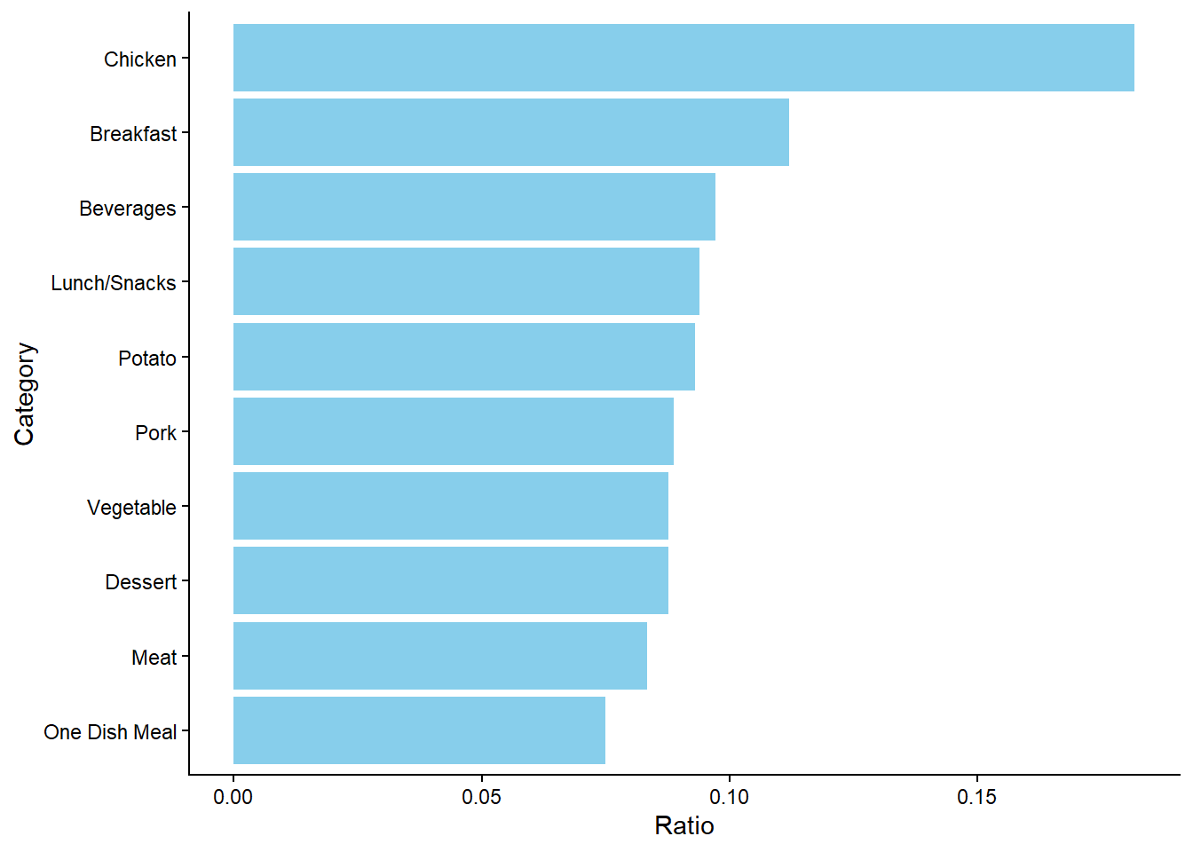
The numeric variable Calories is a numeric variable whose distribution is worth to look at. The graph below shows that the distribution is right-skewed, something that would suggest that it may be needed to perform log transformation in the predictive modeling process.
# Calories Distribution
data %>%
  ggplot(aes(x = Calories)) +
  geom_histogram(fill = "blue") +
  ylab("skyblue")
`stat_bin()` using `bins = 30`. Pick better value `binwidth`.Warning: Removed 52 rows containing non-finite outside the scale range
(`stat_bin()`).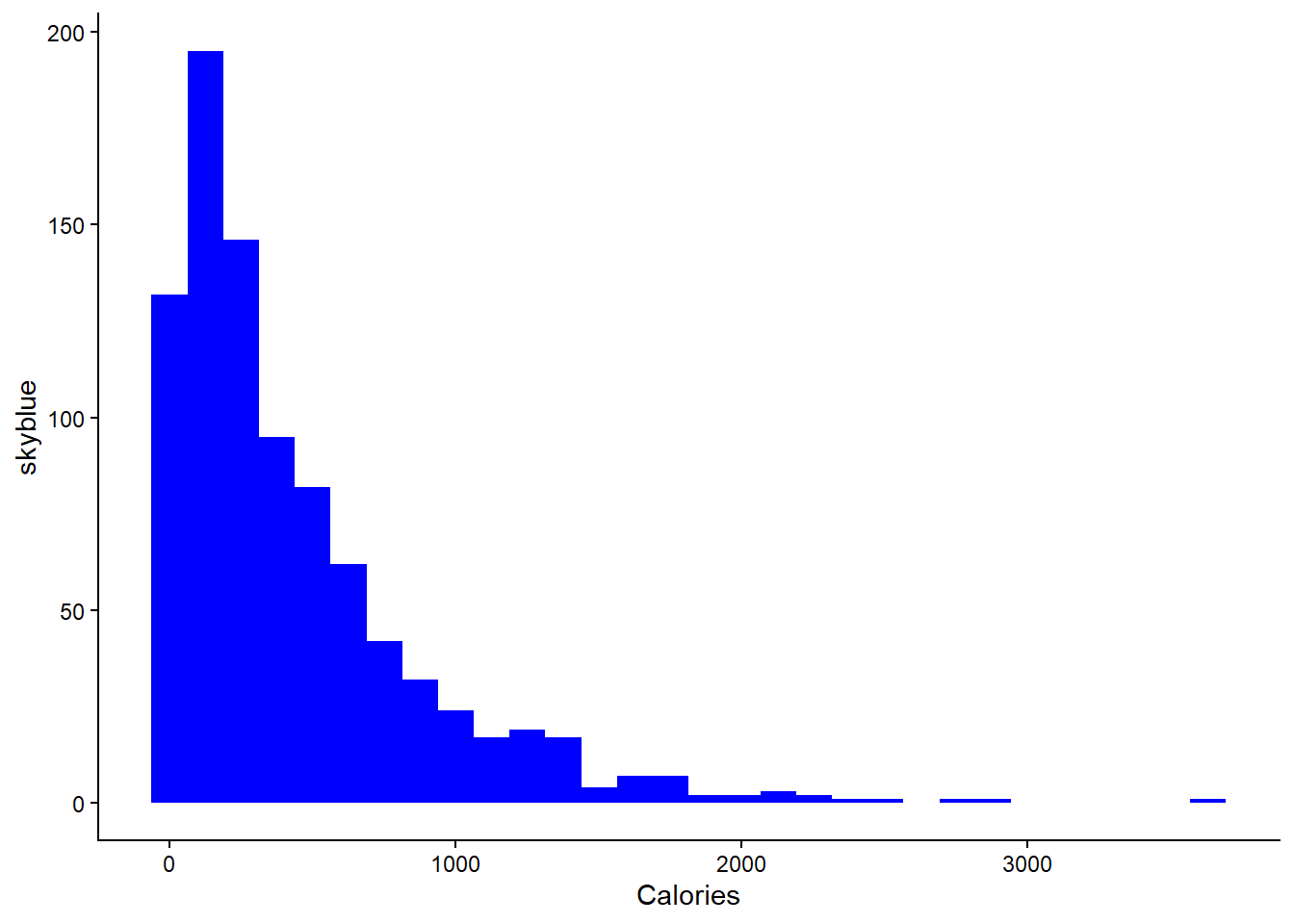
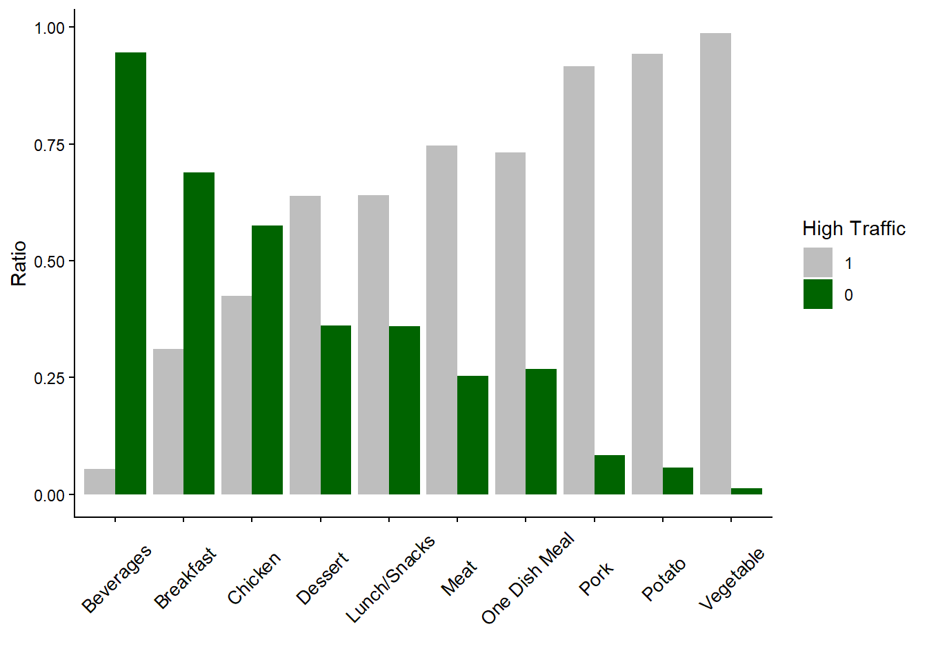
The graph below clearly shows the relationship between the variable Category and the variable High_Traffic. Surprisingly, recipes of “Potato” and “Vegetable” have a higher chance to lead to high traffic when we compare them with categories such as “Chicken” or “Beverages”, categories that captures a high ratio of the recipes. Based on this graph, the business might be able to increase the traffic if more recipes of “Vegetable” or “Potato” are provided.
# High Traffic within Category
data %>%
  count(High_Traffic, Category) %>%
  group_by(Category) %>%
  mutate(Ratio = n/sum(n)) %>%
  ggplot(aes(x = Category,
             y = Ratio,
             fill = High_Traffic)) +
  geom_col(position = "dodge") +
  scale_fill_manual(values = c("grey", "darkgreen")) +
  theme(axis.text.x = element_text(angle = 45,
                                   vjust = 0.5,
                                   size = 10)) +
  labs(
    x = "",
    fill = "High Traffic"
  )
Predictive Modeling
Model Selection and Problem Type
Since the problem was related to whether a recipe is associated with high traffic, it is considered a classification problem with two classes: high traffic (value of 1) or not high traffic (value of 0). Two predictive modeling methodologies that are appropriate for this type of problem are Logistic Regression and Random Forest. The first can be seen as a simpler methodology that requires more complex data pre-processing while the second can be viewed as a black box methodology that does not require much data pre-processing. At the same time, these methodologies are not similar to each other, meaning that they can capture different patterns in the data (Kuhn & Kjell, 2019). As random forest is considered more complex methodology, logistic regression will be used for the baseline model and random forest will be utilized for the comparison model.
# Set seed
set.seed(123)

# Split the data set
data_split <- initial_split(data = data,
                            prop = 0.75,
                            strata = High_Traffic)
training_set <- data_split %>% training()
test_set <- data_split %>% testing()
Fitting the baseline and comparison models
As mentioned, logistic regression and random forest were chosen as methodologies. Because we use tidymodels, we initiate the engines, by clarifying that the task (mode) is classification and using the packages glmnet and ranger. For the first, I tuned the parameter lambda, whose argument name in the function is “penalty” and which essentially gives a penalty for coefficients that are too high. The purpose is to introduce some bias in the modeling process in order to decrease the variance and, as a result, make sure that the model does not overfit the training data. For the random forest model, we specified that the forest will consist of 2000 trees. During each data split, the algorithm randomly selects 2 variables as candidates for the split. Additionally, we tune the parameter that specifies the minimum node size of a tree, which determines the minimum number of observations required for a potential additional split to occur.
# Logistic Regression - Initiate Engine
lr_model <- logistic_reg(mode = "classification",
                         penalty = tune()) %>%
  set_engine("glmnet")

# Random Forest - Initiate Engine
rf_model <- rand_forest(mode = "classification",
                        trees = 2000,
                        mtry = 2,
                        min_n = tune()) %>%
  set_engine("ranger")
In both models, we impute the missing values on all numeric predictors via a linear model and we transform the variable Category from a categorical variable to dummy variables in order to have a dummy variable for each category (except one to avoid perfect collinearity). For logistic regression, we also use log transformation on the variable Calories (after the mentioned linear imputation).
# Logistic Regression Recipe
lr_recipe_data <- recipe(High_Traffic ~ .,
                         data = training_set %>% select(-Recipe)) %>%
  step_impute_linear(c(Calories, Carbohydrates, Sugar, Protein),
                     impute_with = imp_vars(Servings, Category)) %>%
  step_log(Calories) %>%
  step_dummy(all_nominal_predictors())

# Random Forest Recipe
rf_recipe_data <- recipe(High_Traffic ~ .,
                         data = training_set %>% select(-Recipe)) %>%
  step_impute_linear(c(Calories, Carbohydrates, Sugar, Protein),
                     impute_with = imp_vars(Servings, Category)) %>%
  step_dummy(all_nominal_predictors())
For tuning, we follow a regular grid approach, considering 20 potential values for each hyperparameter of every model. Specifically, for the logistic regression model, the grid encompassed penalty values, while for the random forest model, the grid comprised different values representing the minimum number of observations required for a split to occur.
# Logistic Regression Grid
lr_grid <- grid_regular(extract_parameter_set_dials(lr_model),
                        levels = 20)

# Random Forest Grid
rf_grid <- grid_regular(extract_parameter_set_dials(rf_model),
                        levels = 20)
To combine each recipe with the corresponding model, I created two separate workflows (based on the tidymodels functionality) to combine each model with its corresponding recipe.
# Logistic Regression Workflow
lr_workflow <- workflow() %>%
  add_model(lr_model) %>%
  add_recipe(lr_recipe_data)

# Random Forest Workflow
rf_workflow <- workflow() %>%
  add_model(rf_model) %>%
  add_recipe(rf_recipe_data)
For training, we use the k-fold cross validation method. More specifically, we split the data set into 10 different folds (so k is 10). Each model is going to be trained in 9 out of 10 folds and then tested on the 10th fold (the one that was left out). This process occurs 10 times and so each model will be tested in all 10 folds as a result.
# Set seed
set.seed(321)

# Create 10-fold cross validation
data_folds <- vfold_cv(training_set, v = 10)
The goal of this project is to create a predictive model that is able to “predict which recipes will lead to high traffic and correctly predict high traffic recipes 80% of the time”. From this statement, we understand that the business is interested in the metrics recall and precision. The first is about finding the recipes that are actually of high-traffic. In other words, if 10 recipes lead to high traffic, the model should be able to predict most of them. The latter reflects the success rate on the recipes that are selected by the business as of high-traffic. Put differently, if 10 recipes are selected (based on the selected model) to be of high-traffic, at least 8 (or 80%) should actually be of high-traffic.
We mention these metrics here because we use them to evaluate the predictive models in the training phase. Therefore, having these metrics in mind, we tune the parameters and applied cross validation with each model separately.
# Logistic Regression - Training
set.seed(123)
lr_results <- lr_workflow %>%
  tune_grid(resamples = data_folds,
            grid = lr_grid,
            metrics = metric_set(recall, precision))

# Random Forest - Training
set.seed(123)
rf_results <- rf_workflow %>%
  tune_grid(resamples = data_folds,
            grid = rf_grid,
            metrics = metric_set(recall, precision))
To check the performance of the two models, we use a line plot to check the average precision and average recall per value of the tuned hyperparameter.
# Logistic Regression - Precision and Recall
autoplot(lr_results)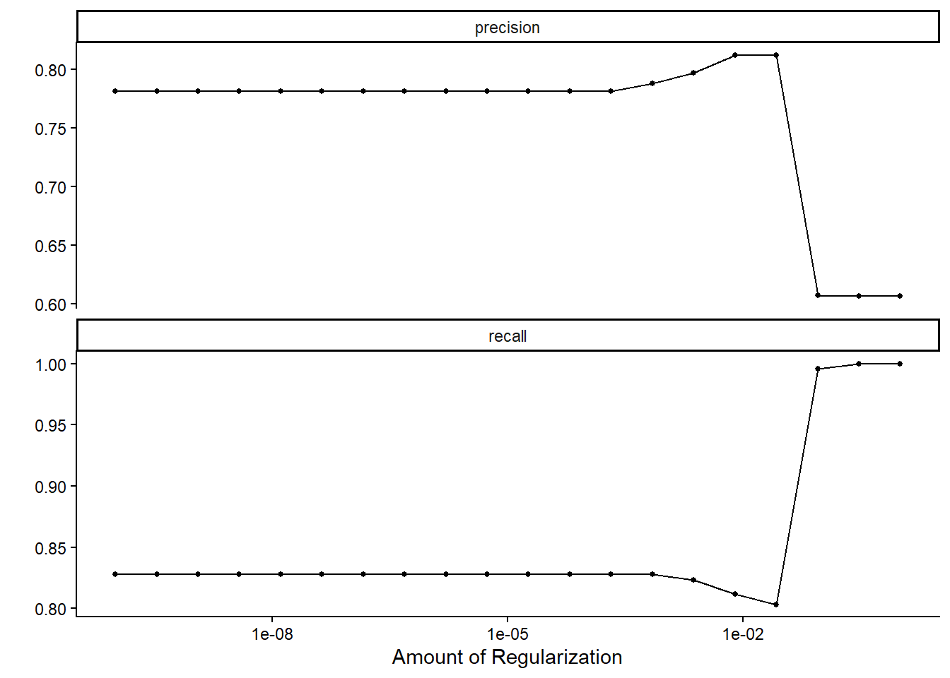
# Random Forest - Precision and Recall
autoplot(rf_results)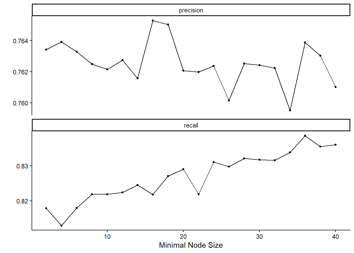
The degree of regularization in the logistic regression models does not substantially affect recall or precision in most cases. However, when the regularization strength becomes relatively large, recall increases to 100%, at the cost of a marked reduction in precision. A recall of 100% implies that the model classifies every observation as leading to high traffic, thereby ensuring that all truly high-traffic cases are captured, but at the expense of generating many false positives.
In contrast, the random forest models display higher recall values as the minimal node size increases, while precision varies across different node size settings.
Since both precision and recall are critical for the business context, it is necessary to consider their trade-off when selecting the final model. By considering both business acceptance criteria, we retain the logistic regression model with a regularization parameter of approximately 0.026, which yields a precision of around 80%. Also, we select the random forest model with a minimal node size of 21.
The performance metrics of the selected models are as follows:
# Logistic Regression - Metric values of chosen version
lr_results %>%
  collect_metrics() %>%
  filter(penalty > 0.0263 & penalty < 0.0265)
# A tibble: 2 × 7
penalty .metric .estimator mean n std_err .config
<dbl> <chr> <chr> <dbl> <int> <dbl> <chr>
1 0.0264 precision binary 0.812 10 0.0272 pre0_mod17_post0
2 0.0264 recall binary 0.803 10 0.0140 pre0_mod17_post0# Random Forest - Metric values of chosen version
rf_results %>%
collect_metrics() %>%
filter(min_n == 28)# A tibble: 2 × 7
min_n .metric .estimator mean n std_err .config
<int> <chr> <chr> <dbl> <int> <dbl> <chr>
1 28 precision binary 0.763 10 0.0259 pre0_mod14_post0
2 28 recall binary 0.832 10 0.0112 pre0_mod14_post0The random forest model achieves higher recall but lower precision, whereas the logistic regression model provides a more balanced performance across the two metrics.
The next step is to evaluate how these models perform on the test set. To do so, we compare the predicted outcomes with the actual values by examining the confusion matrices of each model, alongside their corresponding precision and recall scores.
# Logistic Regression - Choose Model
chosen_lr_model <- lr_results %>%
  collect_metrics() %>%
  filter(penalty > 0.0263 & penalty < 0.0265) %>%
  slice(1)

# Logistic Regression - Confusion Matrix
set.seed(123)
lr_workflow %>%
  finalize_workflow(chosen_lr_model) %>%
  last_fit(split = data_split) %>%
  collect_predictions() %>%
  conf_mat(truth = High_Traffic, .pred_class)
Truth
Prediction 1 0
1 115 35
0 29 59# Logistic Regression - Recall
set.seed(123)
lr_workflow %>%
finalize_workflow(chosen_lr_model) %>%
last_fit(split = data_split) %>%
collect_predictions() %>%
recall(truth = High_Traffic, .pred_class)# A tibble: 1 × 3
.metric .estimator .estimate
<chr> <chr> <dbl>
1 recall binary 0.799# Logistic Regression - Precision
set.seed(123)
lr_workflow %>%
finalize_workflow(chosen_lr_model) %>%
last_fit(split = data_split) %>%
collect_predictions() %>%
precision(truth = High_Traffic, .pred_class)# A tibble: 1 × 3
.metric .estimator .estimate
<chr> <chr> <dbl>
1 precision binary 0.767# Random Forest - Choose Model
chosen_rf_model <- rf_results %>%
collect_metrics() %>%
filter(min_n == 28) %>%
slice(1)
# Random Forest - Confusion Matrix
set.seed(123)
rf_workflow %>%
finalize_workflow(chosen_rf_model) %>%
last_fit(split = data_split) %>%
collect_predictions() %>%
conf_mat(truth = High_Traffic, .pred_class) Truth
Prediction 1 0
1 123 40
0 21 54# Random Forest - Recall
set.seed(123)
rf_workflow %>%
finalize_workflow(chosen_rf_model) %>%
last_fit(split = data_split) %>%
collect_predictions() %>%
recall(truth = High_Traffic, .pred_class)# A tibble: 1 × 3
.metric .estimator .estimate
<chr> <chr> <dbl>
1 recall binary 0.854# Random Forest - Precision
set.seed(123)
rf_workflow %>%
finalize_workflow(chosen_rf_model) %>%
last_fit(split = data_split) %>%
collect_predictions() %>%
precision(truth = High_Traffic, .pred_class)# A tibble: 1 × 3
.metric .estimator .estimate
<chr> <chr> <dbl>
1 precision binary 0.755As expected, the random forest model achieves higher recall but lower precision compared to the logistic regression model. However, the difference is relatively small: the recall of the random forest model is nearly three percentage points higher, while its precision is only about one percentage point lower than that of the logistic regression model.
In terms of individual cases, the random forest model correctly identifies four additional high-traffic recipes, whereas the logistic regression model correctly classifies three additional low-traffic recipes.
Given that the two models are very similar in terms of overall performance, it is not immediately clear which should be preferred. Logistic regression offers the advantage of simplicity and a slightly better balance between recall and precision, while the random forest model demonstrates somewhat greater stability on the test set. The ultimate choice depends on the business context and whether capturing more high-traffic cases or avoiding false positives is considered more critical.
Business Metrics
The company can use Website Visits as the main KPI to evaluate model performance against the stated business objectives. As a starting point, the business could compare the predicted outcomes of the models with the average number of visits for each traffic level (high vs. not high traffic). For instance, if a predictive model classifies a recipe as leading to high traffic, the number of visits generated by that recipe can be compared to the current average number of visits for high-traffic recipes.
For the logistic regression model, we would expect that most recipes predicted as high traffic would generate visit counts close to the existing average for high-traffic recipes. This aligns with the model’s balanced performance between precision and recall, meaning it is relatively good both at capturing true high-traffic cases and at avoiding false positives.
For the random forest model, we would expect a slightly higher proportion of correctly identified high-traffic recipes—around 83%—and in absolute terms, this model correctly captures four more high-traffic recipes than logistic regression. However, this comes at the expense of slightly lower precision, as the model also includes more false positives in its predictions.
Because the performance of the two models is very close overall, the choice between them ultimately depends on business priorities: logistic regression offers interpretability and a balanced trade-off, while random forest provides a small advantage in recall and has shown more stability on the test set. In practice, the business could also assess the impact of each model by comparing website visits before and after implementation (A/B testing), or even by running both models in parallel to evaluate which yields greater business value in real-world use.
Final Summary and Recommendations
The goal of this project was to analyze which recipes are most likely to generate high website traffic. Data exploration and visualization showed that more than 50% of the recipes fall into the high-traffic category, with recipes based on vegetables, potatoes, and pork performing particularly well compared to other food types.
To predict which recipes will lead to high traffic, two predictive models were developed: a logistic regression model and a random forest model. On the unseen test data, the models produced very similar overall performance, but with slightly different trade-offs. The logistic regression model demonstrated a more balanced performance between precision and recall, whereas the random forest model achieved marginally higher recall (capturing four additional high-traffic recipes) at the cost of slightly lower precision. In addition, the random forest model appeared somewhat more stable in its test-set predictions.
Because both recall and precision are important for the business, the choice between the two models depends on strategic priorities. Logistic regression may be preferred if interpretability and balance between metrics are valued, while the random forest model may be better suited if maximizing the capture of high-traffic recipes is the primary objective.
The company can use Website Visits as the main KPI to evaluate the impact of implementing either model. For instance, traffic levels predicted as “high” can be compared to the historical average number of visits for high-traffic recipes. Furthermore, the business could track changes in average website visits before and after implementation (A/B testing) to quantify the added value of predictive modeling.
References
Kuhn, M., & Johnson, K. (2019). Feature engineering and selection: A practical approach for predictive models. Taylor & Francis/CRC Press.